Majority Voting

Majority Voting

Problem

Here’s a problem that comes up very often in computer science. Let’s say you have some process that gives you the right answer **most** of the time, but not always. For example: you need to check if a particular transaction is “final” in a block chain. To keep things simple we’ll consider only “true or false” kind of questions. Let’s say the probability of getting the **wrong** answer is \(f \le 1/2\).

Obviously, you want the probability of getting things right to be a lot better than a half, so you run the process \(n\) times independently, and then if the majority of the answers are true then you say the result is true, and false otherwise. How many times do you need to run the process (i.e. what must \(n\) be) in order to get the correct answer with probability at least \(1 - \delta\)?

This is called the “Majority Voting” problem, and while there are several ways to analyse it. Usually a few simplifying assumptions are made and people just fast-forward to the bottom line that \(n \ge O \left( \log \frac{1}{\delta} \right)\). While this is true, it hides the effect of all of the constants. How close can \(f\) be to \(1/2\)?

I’m going to present an analysis here that uses as few approximations as possible so that we can study the effect of the constants at the end. It’s fairly detailed, but serves as a good example of how to do this kind of analysis.

Solution

Since we’re looking for a majority, we’ll assume that we do an odd number of trials, i.e. \(n = 2t + 1\). We can model this problem as a series of coin tosses, each with a probability of coming up tails \(f\), and asking what is the probability that you get heads \(t+1\) times or more? The probability of any particular combination of heads and tails can be modelled as a Binomial Distribution. Consider the probability that we get **exactly** \(t + 1\) tails:

\[\Pr\left[t + 1 \text{ tails}\right] = {2t + 1 \choose t + 1} f^{t+1} (1-f)^{t} = p\]

Let \(f = \frac{1-\varepsilon}{2}\) and rearrange a bit:

\[\begin{split} \Pr\left[t + 1 \text{ tails}\right] &= \frac{(2t + 1)!}{(t + 1)!t!} \cdot f \cdot \left(\frac{1-\varepsilon}{2}\right)^{t} \left(\frac{1+\varepsilon}{2}\right)^{t} \\ &= \frac{2t+1}{t+1}f \cdot \frac{(2t)!}{(t!)^2} \cdot \left(\frac{1 - \varepsilon^2}{2^2}\right)^t \end{split}\]

Let \(k = 1 - \varepsilon^2\)

\[\Pr\left[t + 1 \text{ tails}\right] = \frac{2t+1}{t+1}f \cdot \frac{(2t)!}{(t!)^2} \cdot \left(\frac{k}{2^2}\right)^t\]

Stirling’s Formula (see this lecture):

\[n! = \sqrt{2 \pi n} \cdot \frac{n^n}{e^n} \cdot \left(1 \pm O(1/n) \right)\]

Applying this to the above:

\[\frac{(2t)!}{(t!)^2} = \frac{\sqrt{2 \pi 2t} \cdot \left( \frac{2t}{e} \right)^{2t} \cdot \left(1 \pm O(1/n) \right)}{\left( \sqrt{2 \pi t} \cdot \left( \frac{t}{e} \right)^{t} \cdot \left(1 \pm O(1/n) \right) \right)^2} \sim \frac{2^{2t}}{\sqrt{\pi t}}\]

Notice that a lot of things cancel out. We’ll assume the error terms cancel out as well, which is true asymptotically. Substituting back, we get:

\[\Pr\left[t + 1 \text{ tails}\right] \sim \frac{2t+1}{t+1}f \cdot \frac{2^{2t}}{\sqrt{\pi t}} \cdot \left(\frac{k}{2^2}\right)^t = \frac{2t+1}{t+1}f \cdot \frac{k^t}{\sqrt{\pi t}}\]

Now consider what happens if we get more failures:

\[\begin{split} \Pr[t + 1 + i \text{ tails}] &= {2t + 1 \choose t + 1 + i} f^{t+i+1} (1-f)^{t - i} \\ &= \frac{(2t + 1)!}{(t + 1 + i)!(t - i)!} f^{t+1} (1-f)^t f^i (1-f)^{-i} \\ &= \frac{(2t + 1)!}{ (t + 1)! t!} f^{t+1} (1-f)^t \frac{(t - i + 1) \cdots t}{(t + 1 + i) \cdots (t + 2)} \left(\frac{f}{1-f}\right)^{i} \end{split}\]

Notice that the left side is exactly \(p\) defined above. As for the right side, notice that \(\forall x > 0, i > 0\):

\[\frac{x}{x+1} > \frac{x - i}{x + 1 + i}\]

We can substitute this into the middle terms.

Let \(\alpha = \frac{t}{t + 2} \frac{f} {1 - f}\)

\[\Pr[t + 1 + i \text{ tails}] \le \frac{(2t + 1)!}{ (t + 1)! t!} f^{t+1} (1-f)^t \left(\frac{t}{t + 2}\frac{f}{1-f}\right)^{i} = p\alpha^i\]

We can now bound the overall probability of failure:

\[\begin{split} \Pr\left[\text{failure}\right] &= \Pr[t + 1 \text{ tails}] + \Pr[t + 2 \text{ tails}] + \ldots \Pr[2t + 1 \text{ tails}] \\ &\le p + \alpha p + \ldots \alpha^t p \end{split}\]

Notice that this is simply a geometric series.

\[\Pr\left[\text{failure}\right] \le p \frac{1 - \alpha^{t}}{1 - \alpha} \le \frac{2t+1}{t+1}f \cdot \frac{k^t}{\sqrt{\pi t}} \cdot \frac{1 - \alpha^{t}}{1 - \alpha}\]

To simplify things a bit:

\[\frac{1-\alpha^t}{1-\alpha} \le \frac{1}{1-\alpha}\]

We can also get rid of the first term as for \(f < 1/2, t > 0\):

\[\frac{2t+1}{t+1}f \le \frac{t + 1/2}{t + 1} < 1\]

The problem reduces to:

\[\Pr\left[\text{failure}\right] \le \frac{k^t}{\sqrt{\pi t}} \cdot \frac{1}{1 - \alpha}\]

Substitute for \(\alpha = \frac{t}{t + 2} \frac{f} {1 - f} = \frac{t}{t + 2} \frac{1 - \varepsilon}{1 + \varepsilon}\)

\[\Pr\left[\text{failure}\right] \le \frac{k^t}{\sqrt{\pi t}} \cdot \frac{(t + 2)(1 + \varepsilon)}{2(t \varepsilon + \varepsilon + 1)}\]

If we fix some \(0 < \varepsilon < 1\) then the right side of this converges to a constant value (and pretty quickly if \(\varepsilon\) isn’t very close to zero). We’ll analyse that in more detail later, for now let’s replace it with a constant and assume that \(k\) is also some constant value too. Then notice that for large enough \(t\) the denominator can be replaced by a constant too. We can simplify and apply our desired bound.

\[\Pr\left[\text{failure}\right] \le \frac{c' k^t}{\sqrt{\pi t}} \le c k^t \le \delta\]

Taking log of both sides:

\[t \log k + \log c \le \log \delta\] \[t \ge \frac{\log \frac{1}{\delta} + \log c}{\log \frac{1}{k}}\]

Which we can state more simply as:

\[t \ge O\left( \log \frac{1}{\delta} \right)\]

Effect of \(\varepsilon\)

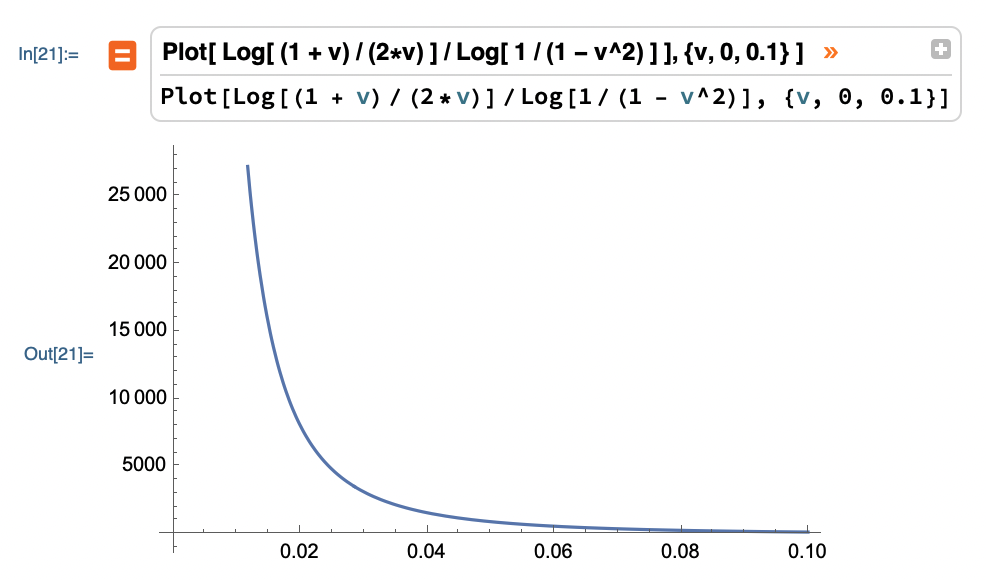
The analysis above works really well if we assume that \(\varepsilon\) is some fixed value greater than zero. But you may notice that if it’s very close to zero, things stop working. Consider the constant we threw out:

\[c = \frac{(t + 2)(1 + \varepsilon)}{2(t \varepsilon + \varepsilon + 1)}\]

Notice what happens as \(t\) goes to infinity:

\[\lim_{t \rightarrow \infty} c = \lim_{t \rightarrow \infty} \frac{(1 + 2/t)(1 + \varepsilon)}{2(\varepsilon + \varepsilon/t + 1/t)} = \frac{1 + \varepsilon}{2 \varepsilon}\]

In other words, as epsilon gets arbitrarily small our constant goes asymptotically to infinity!

What about the \(k\) value in the denominator? Let’s expand that:

\[\log \frac{1}{1 - \varepsilon^2}\]

On the flipside, this produces exponentially smaller values as \(\varepsilon\) gets small, which in the denominator make things grow exponentially! Here’s what it looks like:

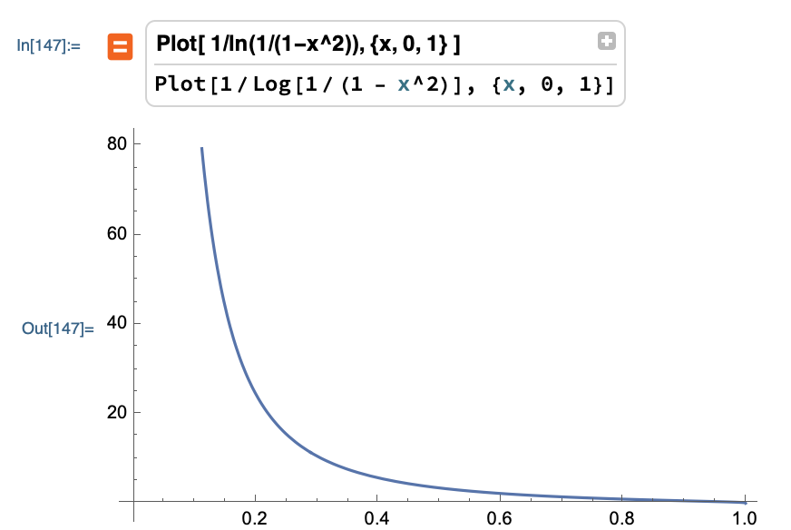
This by itself when applied to \(\delta\) is problematic. When combined with the effect on the constant term, you get a rather huge explosion!

Conclusions

The analysis usually given that \(n \ge O \left( \log \frac{1}{\delta} \right)\) is correct for reasonable values of \(\varepsilon\), but don’t forget to analyse your constants! In this case, if \(\varepsilon\) gets very small, the constant values explode very badly.

This makes sense when you think about it. You’re essentially trying to distinguish two distributions: correct and incorrect responses. If the two are arbitrarily close to each other, you can’t distinguish without taking an arbitrarily large number of samples. If the two are far apart, you can distinguish them in a much smaller number of samples.